Category:Robotic
Here you can find a very brief overview of robots used in manufacturing. It talks about what is it that makes a machine a robot, what differentiates the various types of robots, different ways robots can move, and three types of power sources for robots.
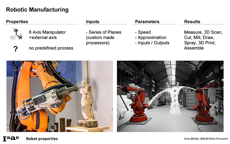
Robot properties
Contents
Terminology
Karl Capek coined the term robot in 1920. He was a Czech playwright who wrote R.U.R. which stands for Rosumovi Univerzální Roboti (Rossum’s Universal Robots).
The term robot might comes from the Czech words robota and robotník, which literally means "work" and "worker" respectively. However, the word robota also means "work" or "serf labour" in Slovak.
Modern definition of a robot
Encyclopedia Britannica's definition of a robot is as follows:
"Any automatically operated machine that replaces human effort, though it might not resemble human beings in appearance or perform functions in a humanlike manner."
The Robotics Primer (which we also highly recommend), Maja J. Mataric uses the following definition:
"A robot is an autonomous system which exists in the physical world, can sense its environment, and can act on it to achieve some goals."
Another definition by Lentin Joseph in Learning Robotics Using Python, 2015 :
"A robot is an autonomous system which exists in the physical world, can sense its environment, and can act on it to achieve some goals."
History
(Chapter extracted from the book "Learning Robotics Using Python, Lentin Joseph, 2015.")
It's quite difficult to pinpoint a precise date in history, which we can mark as the date of birth of the first robot. For one, we have established quite a restrictive definition of a robot previously; thus, we will have to wait until the 20th century to actually see a robot in the proper sense of the word. Until then, let's at least discuss the honourable mentions.
The first one that comes close to a robot is a mechanical bird called "The Pigeon". This was postulated by a Greek mathematician Archytas of Tarentum in the 4th century BC and was supposed to be propelled by steam. It cannot be considered a robot by our definition (not being able to sense its environment already disqualifies it), but it comes pretty comes for its age. Over the following centuries, there were many attempts to create automatic machines, such as clocks measuring time using the flow of water, life-sized mechanical figures, or even first programmable humanoid robots (it was actually a boat with four automatic musicians on it). The problem with all these is that they are very disputable as there is very little (or none) historically trustworthy information available about these machines.
It would have stayed like this for quite some time if it was not for Leonardo Da Vinci's notebooks that were rediscovered in the 1950s. They contain a complete drawing of a 1945 humanoid (a fancy word for a mechanical device that resembles humans), which looks like an armoured knight. It seems that it was designed so that it could sit up, wave its arms, move its head, and most importantly, amuse royalty. In the 18th century, following the amusement line, Jacques de Vaucanson created three automata: a flute player that could play twelve songs, a tambourine player, and the most famous one, "The Digesting Duck". This duck was capable of moving, quacking, flapping wings, or even eating and digesting food (not in a way you will probably think—it just released matter stored in a hidden compartment). It was an example of "moving anatomy"—modeling human or animal anatomy using mechanics.
Our list will not be complete if we omitted these robot-like devices that came about in the following century. Many of them were radio-controlled, such as Nikola Tesla's boat, which he showcased at Madison Square Garden in New York. You could command it to go forward, stop, turn left or right, turn its lights on or off, and even submerge. All of this did not seem too impressive at that time because the press reports attributed it to "mind control".
At this point, we have once again reached the time when the term robot was used for the first time. As we said many times before, it was in 1920 when Karel Čapek used it in his play, R.U.R. Two decades later, another very important term was coined. Issac Asimov used the term robotics for the first time in his story "Runaround" in 1942. Asimov wrote many other stories about robots and is considered to be a prominent sci-fi author of his time.
However, in the world of robotics, he is known for his three laws of robotics:
• First law: A robot may not injure a human being or through inaction allow a human being to come to harm.
• Second Law: A robot must obey the orders given to it by human beings, except where such orders would conflict with the first law.
• Third law: A robot must protect its own existence, as long as such protection does not conflict with the first or second law.
After a while, he added a zeroth law:
• Zeroth law: A robot may not harm humanity or by inaction allow humanity to come to harm.
These laws somehow reflect the feelings people had about machines they called robots at that time. Seeing enslavement by some sort of intelligent machine as a real possibility, these laws were supposed to be some sort of guiding principles one should at least keep in mind, if not directly follow when designing a new intelligent machine. Also, while many were afraid of the robot apocalypse, the time has shown that it's still yet to come. In order for it to take place, machines will need to get some sort of intelligence, some ability to think and act based on their thoughts. Also, while we can see that over the course of history, the mechanical side of robots went through some development, the intelligence simply was not there yet. This was part of the reason why in the summer of 1956, a group of very wise gentlemen (which included Marvin Minsky, John McCarthy, Herbert Simon, and Allan Newell) was later called to be the founding fathers of the newly founded field of Artificial Intelligence. It was at this very event where they got together to discuss creating intelligence in machines (thus, the term artificial intelligence).
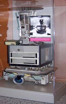
Although, their goals were very ambitious (some sources even mention that their idea was to build this whole machine intelligence during that summer), it took quite a while until some interesting results could be presented. One such example is Shakey, a robot built by the Stanford Research Institute (SRI) in 1966. It was the first robot (in our modern sense of the word) capable to reason its own actions. The robots built before this usually had all the actions they could execute preprogrammed. On the other hand, Shakey was able to analyze a more complex command and split it into smaller problems on his own.
The following image of Shakey is taken from https://en.wikipedia.org/wiki/ File:ShakeyLivesHere.jpg:
Shakey, resting in the Computer History Museum in Mountain View, California
His hardware was quite advanced too. He had collision detectors, sonar range finders, and a television camera. He operated in a small closed environment of rooms, which were usually filled with obstacles of many kinds. In order to navigate around these obstacles, it was necessary to find a way around these obstacles while not bumping into something. Shakey did it in a very straightforward way.
At first, he carefully planned his moves around these obstacles and slowly (the technology was not as advanced back then) tried to move around them. Of course, getting from a stable position to movement wouldn't be possible without some shaky moves. The problem was that Shakey's movements were mostly of this shakey nature, so he could not be called anything other than Shakey. The lessons learned by the researchers who were trying to teach Shakey how to navigate in his environment turned out to be very important. It comes as no surprise that one of the results of the research on Shakey is the A* search algorithm (an algorithm that can very efficiently find the best path between two goals). This is considered to be one of the most fundamental building blocks not only in the field of robotics or artificial intelligence but also in the field of computer science as a whole. Our discussion on the history of robotics can go on and on for a very long time. Although one can definitely write a book on this topic (as it's a very interesting one), it's not this book; we shall try to get back to the question we tried to answer, which was: where do robots come from?
In a nutshell, robots evolved from the very basic mechanical automation through remotely-controlled objects to devices or systems that can act (or even adopt) on their own in order to achieve some goal. If this sounds way too complicated, do not worry. The truth is that to build your own robot, you do not really need to deeply understand any of this. The vast majority of robots you will encounter are built from simple parts that are not difficult to understand when you see the big picture. So, let's figure out how we will build our own robot. Let's find out what are the robots made of.
Applications
The application is the type of work that the robot is designed to do. Robot models are created with specific applications or processes in mind. Different applications will have different requirements. For instance, a painting robot will require a small payload but a large movement range and be explosion proof. On the other hand, an assembly robot will have a small workspace but will be very precise and fast. Depending on the target application, the industrial robot will have a specific type of movement, linkage dimension, control law, software and accessory packages. Below are some types of applications:
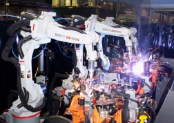
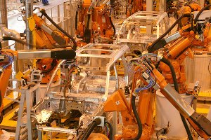
Welding robots
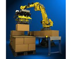
Material handling robots
palletizing robot
Painting robot
Assembly robot
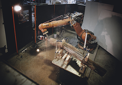
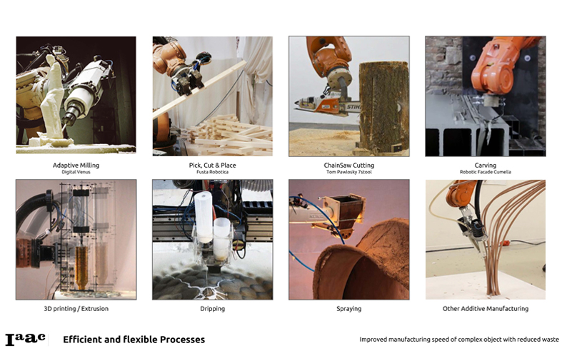
Experimental processes @ IAAC
General principles
Kinematics
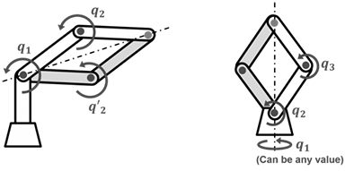
The type of movement is dictated by the arrangement of joints (placement and type) and linkages (Serial or Parallel).
Moreover, taking the article:(Robot Manipulation: Kinematics by Sebastian Castro. 2018) as a definition reference of Kinematics:
It's worth to highlight a quick comparison of kinematics and dynamics:
Kinematics is the analysis of motion without considering forces. Here, we only need geometric properties such as lengths and degrees of freedom of the manipulator bodies.
Dynamics is the analysis of motion caused by forces. In addition to geometry, we now require parameters like mass and inertia to calculate the acceleration of bodies. Robot manipulators are often composed of several joints. Joints are composed of revolute (rotating) or prismatic (linear) degrees of freedom (DOF). Therefore, joint positions can be controlled to place the end effector of the robot in 3D space.
If you know the geometry of the robot and all its joint positions, you can do the math and figure out the position and orientation of any point on the robot. This is known as forwarding kinematics (FK).
The more frequent robot manipulation problem, however, is the opposite. We want to calculate the joint angles needed such that the end effector reaches a specific position and orientation. This is known as inverse kinematics (IK).
Serial
Serial robots are the most common. They are composed of a series of joints and linkages that go from the base to the robot tool.
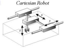
Cartesian robots
Cartesian robots are robots that can do 3 translations using linear slides.
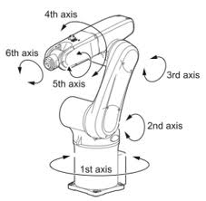
Articulated
In particular 6-axis robots are robots that can fully position their tool in a given position (3 translations) and orientation (3 orientations)
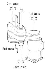
SCARA robots
Scara robots are robots that can do 3 translations plus a rotation around a vertical axis.
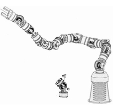
Redundant robots
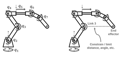
Redundant robots can also fully position their tool in a given position. But while 6-axis robots can only have one posture for one given tool position, redundant robots can accommodate a given tool position under different postures. This is just like the human arm that can hold a fixed handle while moving the shoulder and elbow joints.
Parallel
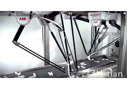
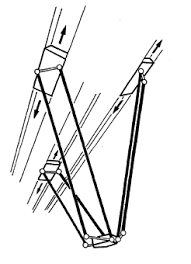
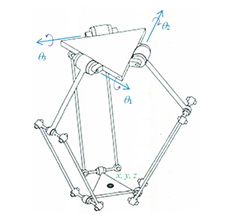
Parallel robots come in many forms. Some call to them spiders robots. Parallel industrial robots are made in such a way that you can close loops from the base, to the tool and back to the base again. It's like many arms working together with the robot tool. Parallel industrial robots typically have a smaller workspace (try to move your arms around while holding your hands together vs the space you can reach with a free arm) but higher accelerations, as the actuators don't need to be moved: they all sit at the base.
Delta or Spider Robot
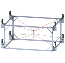
Cable Robot
Others
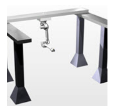
External Axis Linear or Rotary
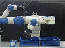
Dual-arm robots Dual-arm robots are composed of two arms that can work together on a given workpiece.
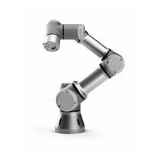
Collaborative industrial robots
There is a new qualifier that has just recently been used to classify an industrial robot, that is to say, if it can collaborate with its human co-workers. Collaborative robots are made in such a way that they respect some safety standards so that they cannot hurt a human. While traditional industrial robots generally need to be fenced off away from human co-workers for safety reasons. Collaborative robots can be used in the same environment as humans. They can also usually be taught instead of programmed by an operator.
Basic terminologies
Work Cell: All the equipment needed to perform the robotic process (robot, table, fixtures, etc.)
Work Envelope: All the space the robot can reach.
Degrees of Freedom: The number of movable motions in the robot. To be considered a robot there needs to be a minimum of 4 degrees of freedom. The Kuka Agilus robots have 6 degrees of freedom.
Payload: The amount of weight a robot can handle at full arm extension and moving at full speed.
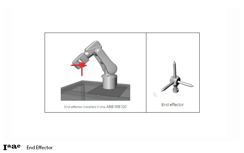
End Effector: The tool that does the work of the robot. Examples: Welding gun, paint gun, gripper, etc.
Manipulator: The robot arm (everything except the End of Arm Tooling).
TCP: Tool Center Point. This is the point (coordinate) that we program in relation to.
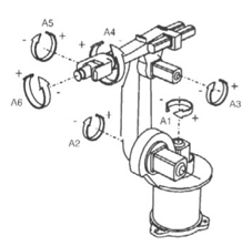
Positioning Axes: The first three axes of the robot (1, 2, 3). Base / Shoulder / Elbow = Positioning Axes. These are the axes near the base of the robot.
Orientation Axes: The other joints (4, 5, 6). These joints are always rotary. Pitch / Roll / Yaw = Orientation Axes. These are the axes closer to the tool.
Coordinates Systems
Types of Motion
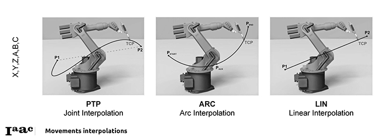
Robot Programming allows us to develop several motion types:
- PTP: POINT TO POINT
The robot guides the TCP along the fastest path to the endpoint. The fastest path is generally not the shortest path and is thus not a straight line. As the motions of the robot axes are rotational, curved paths can be executed faster than straight paths. The exact path of the motion cannot be predicted.
- CIRC: Circular
The robot guides the TCP at a defined velocity along a circular path to the endpoint. The circular path is defined by a start point, auxiliary point and endpoint.
- LIN: Linear
The robot guides the TCP at a defined velocity along a straight path to the end point. This path is predictable.
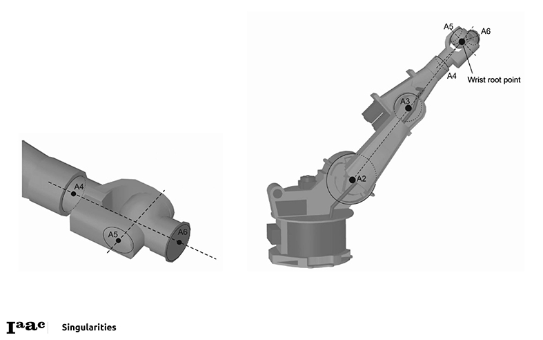
Singularities
(information extracted from Kinematic Singularities - Peter Donelan. Victoria University of Wellington. New Zealand, 2010)
This is a condition in which the manipulator loses one or more degrees of freedom and change in joint variables does not result in change in end effector location and orientation variables. This is a case when the determinant of the Jacobian matrix is zero ie. It is a rank deficit.
Intuitively, Singularities play a significant role in the design and control of robot manipulators. Singularities of the kinematic mapping, which determines the position of the end–effector in terms of the manipulator’s joint variables, may impede control algorithms, lead to large joint velocities, forces and torques and reduce instantaneous mobility.
However they can also enable fine control, and the singularities exhibited by trajectories of the points in the end–effector can be used to mechanical advantage. A number of attempts have been made to understand kinematic singularities and, more specifically, singularities of robot manipulators, using aspects of the singularity theory of smooth maps.
Robot Programming with Kuka|prc
[part of the information explained here is coming from: http://mkmra2.blogspot.com/2016/01/robot-programming-with-kukaprc.html]
KUKA|prc is a set of Grasshopper components that provide Procedural Robot Control for KUKA robots (thus the name PRC). These components are very straightforward to use and it's actually quite easy to program the robots using them.
Rhino File Setup
When you work with the robots using KUKA|prc your units in Rhino must be configured for the Metric system using millimetres. The easiest way to do this is to use the pull-down menus and select File > New... then from the dialogue presented chose "Small Objects - Millimeters" as your template. - Orientation Axes: The other joints (4, 5, 6). These joints are always rotary. Pitch / Roll / Yaw = Orientation Axes. These are the axes closer to the tool.
When installing KUKA|prc has a user interface (UI) much like other Grasshopper plug-ins. The UI consists of the palettes in the KUKA|prc menu.
There are five palettes which organize the components. These are:
01 | Core: The main Core component is here (discussed below). There are also the components for the motion types (linear, spline, etc.). 02 | Virtual Robot: The various KUKA robots are here. We'll mostly be using the KUKA gelis KR6-10 R900 component as those are what are used in the Agilus work cell. 03 | Virtual Tools: Approach and Retract components are here (these determine how the robot should move after a toolpath has completed). There are also components for dividing up curves and surfaces and generating robotic motion based on that division. 04 | Toolpath Utilities: The tools (end effectors) are here. We'll mostly be using the Custom Tool component. 05 | Utilities: The components dealing with input and outputs are stored here. These will be discussed later.
KUKA|prc CORE
The component you always use in every definition is called the Core. It is what generates the KUKA Robot Language (KRL) code that runs on the robot. It also provides the graphical simulation of the robot motion inside Rhino. Everything else gets wired into this component.
The Core component takes five inputs. These are:
SIM- This is a numeric value. Attach a default slider with values from 0.00 to 1.00 to control the simulation.
CMDS- This is the output of one of the KUKA|prc Command components. For example a Linear motion command could be wired into this socket.
TOOL- This is the tool (end effector) to use. It gets wired from one of the Tool components available in the Virtual Tools panel. Usually, you'll use the KUKA|prc Custom Tool option and wire in a Mesh component will show the tool geometry in the simulation.
ROBOT - This is the robot to use. The code will be generated for this robot and the simulation will graphically depict this robot. You'll wire in one of the robots from the Virtual Robot panel. For the Agilus Workcell, you'll use the Agilus KR6-10 R900 component.
COLLISION - This is an optional series of meshes that define collision geometry. Enable collision checking in the KUKA|prc settings to make use of this. Note that collision checking has a large, negative impact on KUKA|prc performance.
There are two output as well:
GEO: This is the geometry of the robot at the current position - as a set of meshes. You can right-click on this socket and choose Bake to generate a mesh version of the robot for any position in the simulation. You can use this for renderings for example.
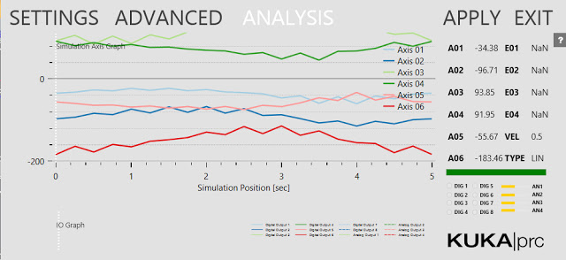
ANALYSIS: This provides a detailed analysis of the simulation values. This has to be enabled for anything to appear. You enable it in the Settings dialogue, Advanced page, Output Analysis Values checkbox. Then use the Analysis component from the Utilities panel. For example, if you wire a Panel component into the Axis Values socket you'll see all the axis values for each command that's run.
Settings
The grey KUKA|prc Settings label at the bottom of the Core component gives you access to its settings. Simply left click on the label and the dialog will appear.
The settings are organized into pages which you select from along the top edge of the dialog (Settings, Advanced, and Analysis). The dialog is modeless which means you can operate Rhino while it is open. To see the effect of your changes in the viewport click the Apply button. These settings will be covered in more detail later.
Basic Setup There is a common set of components used in nearly all definitions for use with the Agilus Workcell. Not surprisingly, these correspond to the inputs on the Core component. Here is a very typical setup:
SIM SLIDER: The simulation Slider goes from 0.000 to 1.000. Dragging it moves the robot through all the motion specified by the Command input. It's often handy to drag the right edge of this slider to make it much wider than the default size. This gives you greater control when you scrub to watch the simulation. You may also want to increase the precision from a single decimal point to several (say 3 or 4). Without that precision, you may not be able to scrub to all the points you want to visualize the motion going through.
You can also add a Play/Pause component. This lets you simulate without dragging the time slider.
CMDS: The components which get wired into the CMDS slot of the Core is really the heart of your definition and will obviously depend on what you are intending the robot to do. In the example above a simple Linear Move, the component is wired in.
TOOL: We normally use custom tools with the Agilus Workcell. Therefore a Mesh component gets wired into the KUKA|prc Custom Tool component (labelled TOOL above). This gets wired into the TOOL slot of the Core. The Mesh component points to a mesh representation of the tool drawn in the Rhino file. See the section below on Tool orientation and configuration.
ROBOT: The robots we have in the Agilus Workcell are KUKA KR6 R900s. So that component is chosen to form the Virtual Robots panel. It gets wired into the ROBOT slot of the Core.
COLLISION: If you want to check for collisions between the robot and the work cell (table) wire in the meshes which represent the work cell. As noted above this has a large negative impact on performance so use this only when necessary.
Robot Position and Orientation
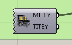
The Agilus workcell has two robots named Mitey and Titey. Depending on which one you are using you'll need to set up some parameters so your simulation functions correctly. These parameters specify the location and orientation of the robot within the workcell 3D model.
Note: The latest revision of Kuka|prc contains a custom robot for the Agilus workcell. It has two output sockets, Mitey and Titey. Simply wire in the robot you intend to use and no more configuration is required.
If you don't have the latest version, see below for how to set them up.
MITEY
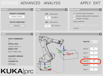
Mitey is the name of the robot mounted in the table. Its base is at 0,0,0. The robot is rotated about its vertical axis 180 degrees. That is, the cable connections are on the right side of the robot base as you face the front of the workcell.
To set up Mitey do the following:
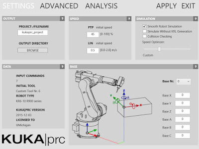
Bring up the Settings dialog by left clicking on KUKA|prc Settings label on the Core component. The dialog presented is shown below:
You specify the X, Y, and Z offsets in the Base X, Base Y, and Base Zdialogues of the dialog. Again, for Mitey these should all be 0. In order to rotate the robot around the vertical axis you specify 180 in the Base A field. You can see that the A axis corresponds to vertical in the diagram.
Base X: 0 Base Y: 0 Base Z: 0 Base A: 180 Base B: 0 Base C: 0
After you hit Apply the robot position will be shown in the viewport. You can close the dialog with the Exit button in the upper right corner.
TITEY
The upper robot hanging from the fixture is named Titey. It has a different X, Y and Z offset values and rotations. Use the settings below when your definition should run on Titey.
Note: These values are all in millimetres. Base X: 1102.5 Base Y: 0 Base Z: 1125.6 Base A: 90 Base B: 180 Base C: 0
Code Output
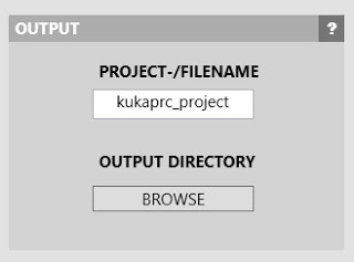
The purpose of KUKA|prc is to generate the code which runs on the robot controller. This code is usually in the Kuka Robot Language (KRL). You need to tell KUKA|prc what directory and file name to use for its code output. Once you've done this, as you make changes in the UI, the output will be re-written as necessary to keep the code up to date with the Grasshopper definition.
To set the output directory and file name follow these steps: Bring up the Settings dialogue via the Core component. On the main Settings page, enter the project filename and choose an output directory. Note: See the? button in the dialogue for recommendations on the filename (which characters to avoid).
Start Position / End Position
When you work with robots there are certain issues you always have to deal with: Reach: Can the robot's arms reach the entire workpiece? Singularities: Will any joint positions result in singularities? (See below for more on this topic) Joint Limits: During the motion of the program will any of the axes hit their limits? One setting which has a major impact on these is the Start Position. The program needs to know how the tool is positioned before the motion starts. This value is VERY important. That's because it establishes an initial placement for the joint limits. Generally, you should choose a start position that doesn't have any of the joints near their rotation limits - otherwise, your programmed path may cause them to hit the joint limit. This is a really common error. Make sure you aren't unintentionally near any of the axes limits. Also, the robot will move from it's current position (wherever that may be) to the start position. It could move right through your workpiece or fixture setup. So make sure you are aware of where the start position is, and make sure there's a clear path from the current position of the robot to the start position. In other words, jog the robot near to the start position to begin. That'll ensure the motion won't hit your set up.
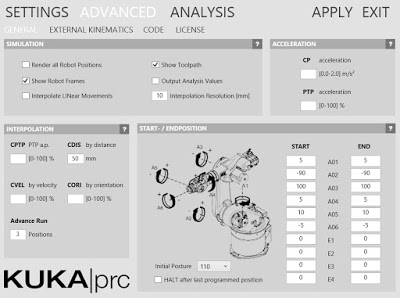
You specify these start and end position values in the Settings of the Core. Bring up the settings dialog and choose the Advanced page.
Under the Start / Endposition section, you enter the axis values for A1 through A6. This begs the questions "how do I know what values to use?".
You can read these directly from the physical robot pendant. That is, you jog the robot into a reasonable start position and read the values from the pendant display. Enter the values into the dialog. Then do the same for the End values. See the section Jogging the Robot in topic Taubman College Agilus Workcell Operating Procedure.
You can also use KUKA|prc to visually set a start position and read the axis values to use. To do this you wire in the KUKA|prc Axis component into the Core component. You can "virtually jog" the robot to a specific position using a setup like this:
Then simply read the axis values from your sliders and enter these as the Start Position or End Position.
Another way is to move the simulation to the start point of the path. Then read the axis values from the Analysis output of the Core Settings dialog. You can see the numbers listed from A01 to A06. Jot these down, one decimal place is fine. Then enter them on the Advanced page.
Initial Posture
Related to the Start Point is the Initial Posture setting. If you've set the Start Position as above and are still seeing motion (like a big shift in one of the axis to reorient) try the As Start option. This sets the initial posture to match the start position.
File:Kuka prc InitialPosture.jpg
Robot Programming with Robots plugin
[part of the information explained here is coming from: https://github.com/visose/Robots/wiki/How-To-Use#grasshopper]
Grasshopper plugin for programming ABB, KUKA and UR robots for custom applications. Special care is taken to have feature parity between all manufacturers and have them behave as similar as possible. The plugin can also be used as a .NET library to create robot programs through scripting inside Rhino (using Python, C# or VB.NET). Advanced functionality is only exposed through scripting.
How To Use
The basic Grasshopper workflow:
1- Select your robot model using the "Load robot" component.
2- Define your end effector (TCP, weight and geometry) using the "Create tool" component.
3- Create a flat list of targets that define your tool path using the "Create target" component.
4- Create a robot program connecting your list of targets and robot model to the "Create program" component.
5- Preview the tool path using the "Simulation" component.
6- Save the robot program to a file using the "Save program" component. If you're using a UR robot, you can also use the "Remote UR" component to stream the program through a network.
Parameters
TARGET
A target defines a robot pose, how to reach it and what to do when it gets there. A tool path is made out of a list of targets. Besides the pose, targets have the following attributes: tool, speed, zone, frame, external axes and commands.
There are two types of targets, joint targets and Cartesian targets:
Joint target: The pose of the robot is defined by 6 rotation values corresponding to the 6 axes. This is the only way to unambiguously define a pose. The first target of a robot program should be a joint target.
Cartesian target: The pose of the robot is defined by a plane that corresponds to the desired position and orientation of the TCP. Cartesian targets can produce singularities, the most common being wrist singularities. This happens when the desired position and orientation requires the 4th and 6th joints to be parallel to each other.
Cartesian targets contain two optional attributes, configuration and motion type:
CONFIGURATION
Industrial robots have 8 different joint configurations to reach the same TCP position and orientation. By default, the configuration in which the joints have to rotate the least is selected. This is determined using the least squares method, which is also the closest distance between targets in joint space. All joints are weighted equally. You can explicitly define a configuration by assigning a value (from 0 to 7) to the Configuration variable. Forcing a configuration doesn't define a pose unambiguously since the joints might rotate clockwise or counter-clockwise depending on the previous target.
Motion type
A robot can move towards a Cartesian target following either a joint motion or a linear motion:
Joint: This is the default motion type. In a joint motion, the controller calculates the joint rotation values on the target using inverse kinematics and moves all of the joints at proportional but fixed speeds so that they will stop at the same time at the desired target. The motion is linear in joint space but the TCP will follow a curved path in world space. It's useful if the path that the TCP follows is not critical, like in pick and place operations. Since inverse kinematics only needs to be calculated at the end of the path, it's also useful to avoid singularities.
Linear: The robot moves towards the target in a straight line in world space. This is useful if the path that the TCP follows is critical, like while milling or extruding material. If the path goes through a singularity at any point it will not be able to continue. If it moves close to a singularity it might slow down below the programmed speed.
Castings
A string containing 6 numbers separated by commas will create a joint target with default attribute values. A plane will create a Cartesian target with default attribute values.
Tool
This parameter defines a tool or end effector mounted to the flange of the robot. In most cases a single tool will be used throughout the tool path, but each target can have a different tool assigned. You might want to change tool if your end effector has more than one TCP, or due to load changes during pick and place. Contains the following attributes:
Name: Name of the tool (should not contain spaces or special characters). The name is used to identify the tool in the pendant and create variable names in post-processing.
TCP: Stand for "tool center point". Represents the position and orientation of the tip of the end effector in relation to the flange. The default value is the world XY plane (the center of the flange).
Weight: The weight of the end effector in kilograms. The default value is 0 kg.
Mesh: Single mesh representing the geometry of the tool. Used for visualization and collision detection.
Coordinate systems
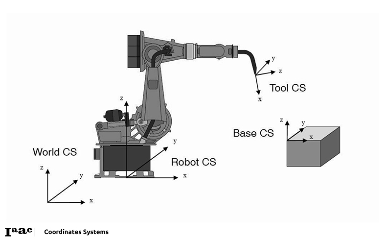
As with Rhino, the plugin uses a right-handed coordinate system. The main coordinate systems are:
World coordinate system: It's the Rhino document's coordinate system. Cartesian robot targets are defined in this system. They've transformed to the robot coordinate system during post-processing.
Robot coordinate system: Used to position the robot in reference to the world coordinate system. By default, robots are placed in the world XY plane. The X axis points away from the front of the robot, the Z axis points vertically.
Tool coordinate system: Used to define the position and orientation of the TCP relative to the flange. The Z axis points away from the flange (normal to the flange), the X axis points downwards.]]
As with Rhino, the plugin uses a right-handed coordinate system. The main coordinate systems are:
World coordinate system: It's the Rhino document's coordinate system. Cartesian robot targets are defined in this system. They have transformed into the robot coordinate system during post-processing.
Robot coordinate system: Used to position the robot in reference to the world coordinate system. By default, robots are placed in the world XY plane. The X axis points away from the front of the robot, the Z axis points vertically.
Tool coordinate system: Used to define the position and orientation of the TCP relative to the flange. The Z axis points away from the flange (normal to the flange), the X-axis points downwards.
Robot
File:ROBOTS create a program.jpg
Represents a specific robot model. It's used to calculate the forward and inverse kinematics for Cartesian targets, to check for possible errors and warnings on a program, for collision detection and simulation. If your robot model is not included in the assembly, check the wiki on how to add your own custom models.
Remote connection: You can use the robot parameter to connect to the robot controller through a network. Currently, this is only supported on UR robots.
Create a program:
Units: The plugin always uses the same units irrespective of the robot type or document settings.
Length: Millimeters
Angle: Radians
Weight: Kilograms
Time: Seconds
Linear speed: Millimeters per second
Angular speed: Radians per second
Uploading the program to a robot
A program defines a complete toolpath and creates the necessary robot code to run it. To create a program you need a list of targets and a robot model.
File:ROBOTS create a program.JPG
When a program is created, the following post-processing is done:
It will clean up and fix common mistakes.
It will run through the sequence of targets checking for kinematic or other errors.
It will return warnings for unexpected behaviour.
It will generate a simulation to preview the toolpath.
It calculates an approximate duration of the program.
If there are no errors, it will generate the necessary code in the robot's native language.
Errors
After the first error is found, it will stop and output a program ending in the error. Most errors are due to kinematics (the TCP not being able to position itself on the target). There are other errors, like exceeding the maximum payload. To identify the error, preview simulation of the program at the last target. Programs that contain errors won't create native code.
Warnings
The program will also inform of any warnings to take into account. Warnings may include changes in configuration, maximum joint speed reached, targets with unassigned values, first target not set as a joint target. Programs that contain warnings will create native code and might be safe to run if the warnings are believed to not cause any issues.
Code
To run the program, a code has to be generated in the specific language used by the manufacturer (RAPID for ABB robots, KRL for KUKA robots and URScript for UR robots). If necessary, this code can then be edited manually. A program containing edited code will not check for warnings or errors and can't be simulated.
Simulation
The program contains a simulation of the tool path. The simulation currently doesn't take into account acceleration, deceleration or approximation zones. It simulates both linear and joint motions, actual robot speed, including slowdowns when moving close to singularities and wait times.
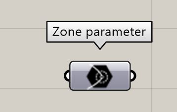
Zone
Defines an approximation zone for a target. Two variables make up a zone, a distance (in mm) and a rotation (in radians). The default value is 0 mm.
Targets can be stop points or way points:
Stop points have a distance and rotation value of 0. All axis will completely before moving to the next target. Commands associated with this target will run just after the TCP reaches the target.
Way points have a distance or rotation value greater than 0. Once the TCP position is within the distance value to the target, it will start moving towards the next target. One the TCP orientation is within the rotation value, it will start orienting towards the next target. This is useful to create a continuous path and avoid the robot stopping (decelerating and accelerating) at the cost of precision. Commands associated with this target will usually run a bit before the TCP enters the zone area.
IMPORTANT: If multiple targets use the same zone, first use a string or number to cast into a zone parameter, then assign the parameter to the different targets. Don't assign a string or number directly as a zone to multiple targets, as different zone instances will be created (even if they have the same value) and will create unnecessary duplication in the robot code.
All the above information comes from the following different sources:
Learning Robotics Using Python, Lentin Joseph. Packt Publishing Ltd, May 27, 2015.
Kinematic Singularities - Peter Donelan. Victoria University of Wellington. New Zealand, 2010
https://github.com/visose/Robots/
and http://mkmra2.blogspot.com/
It should be noted here that the information gathering was drawn by:
Alexandre Dubor,
Kunal Chadha,
Ricardo Mayor Luque
and many people at IAAC
This category currently contains no pages or media.
